What's TDA?

source

• A subfield of algebraic topology that has found applications in many disciplines outside math.
• Based on the idea that data are sampled from an underlying manifold so we can study some algebraic invariants of that space.
• Important algebraic invariant class are homology groups, which arise from combinatorial representations of the manifold.

Simplicial Complexes

• In Euclidean space, a $k$-simplex is the $k$-dimensional convex hull of $k+1$ affinely independent points.
• A simplicial complex is a collection of simplices that are closed under intersection. We can model any topological manifold $\mathbb{X}$ using simplicial complexes.
• The $k$th homology group of $\mathbb{X}$, $H_k(\mathbb{X})$, contains elements that are $k$-cycles but not $k$-boundaries.
• The dimension of $H_k(\mathbb{X})$ is the number of $k$th dimensional holes in $\mathbb{X}$ and is called the $k$th Betti number.

Examples

source

Point cloud

Filtration

As we increase the radii of the balls, we see that holes appear and disappear. Also we note that each prior simplicial complex corresponding to smaller radii is a subcomplex of the new simplicial complex corresponding to the larger radii.

A sequence of simplicial complexes linked by inclusion maps is called a filtration.

Thus, we can keep track of the creation and destruction of topological features of different rank for each complex in the filtration.

Do we always convert data to a point cloud then?

• No, there are different filtrations that can be appropriate for other types of data.
• For example, a nested family of sublevel-sets $f^{-1}((-\infty, \alpha])$ for $\alpha = -\infty$ to $\infty$.
• So we can compute the birth and death connected components and/or holes for filtrations on our data set...

Persistent Homology and Diagrams

For filtered complexes we have that all components are born at the same time. As a younger component meets an older component, the younger one is marked as dead and the two components merge. Note below we also record the birth and death of a 1-d homology group:

source

Persistent Homology and Diagrams

For a single variate function, such as the signal below, we can track and encode the evolution of connected components (0-d homology) of its sublevel-sets:

source

Persistent Homology and Diagrams

Note that we track the components for each $f^{-1}((-\infty, \alpha])$ where $\alpha \in (-\infty, \infty)$. Below we see that components are born at local minima and die at local maxima: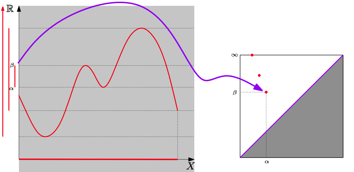

source

Poisson Point Process (PPP)

We will model persistence diagrams as a PPPs. We sample $n$ random points and spatially distribute them. The points are birth and persistence pairs, that is $x_i= (b, p) = (b, d - b), \ i=1,\dots, n$.

The point processes are characterized by the intensity $\lambda(x_i)$, that is the density of the expected number of points at $x_i$.

Marked Poisson Point Process

Def.1) Let $\mathbb{X}$ and $\mathbb{M}$ be Polish spaces. Suppose $\ell : \mathbb{X} \times \mathbb{M} \rightarrow \mathbb{R}^+ \cup \{0\}$ is a function satisfying:

1. $\forall \mathbf{x} \in \mathbb{X}, \ \ell(\mathbf{x}, \cdot)$ is a probability measure on $\mathbb{M}$, and
2. $\forall B \in \mathcal{M}$ (the Borel $\sigma$-algebra of $\mathbb{M}$), $\ell(\cdot, B)$ is a measureable function on $\mathbb{X}$.

Then $\ell$ is a stochastic kernel from $\mathbb{X}$ to $\mathbb{M}$.

Def.2) Let $\Psi_M$ be a finite point process on $\mathbb{X} \times \mathbb{M}$ such that:

1. $\Psi = (\{p_n\}, \{\mathbb{P}_n(\cdot)\})$ is a PPP on $\mathbb{X}$, and
2. for a realization $(\mathbf{x}, \mathbf{m}) \in \mathbb{X} \times \mathbb{M}$, the marks $m_i \in \mathbf{m}$ for each $x_i \in \mathbf{x}$ are independently drawn from a given stochatic kernel $\ell(\cdot, x_i)$.

Then $\Psi_M$ is a marked Poisson point process.

Simple Example

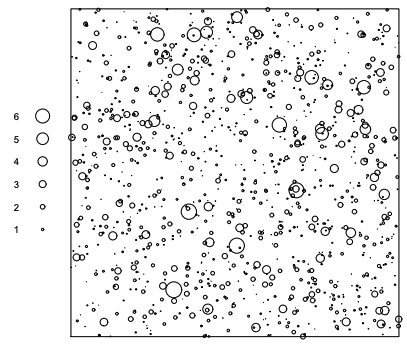
• Generate homogeneous Poisson point process with $\lambda(\mathbf{x}) = 1000$ on $[0,1]^2$.
• Generate $m_i \overset{iid}{\sim}Exp(1)$ at each $\mathbf{x}_i$.
• The marked Poisson point process $\{(\mathbf{x}_i, m_i)\}$ is derived.

source

This is your brain right now...

...ok, now let's talk about the paper...

(link to paper)

Persistent Homology for Noisy Signals

Consider a signal as a bounded and continuous function of time $f(t)$. For every connected component that arises from a sublevel set filtration we plot the points $(b, d)$. We apply a linear combination $(b, p) = (b, d - b)$ and define the set $\mathbb{X} := \{(b, p) \in \mathbb{R}^2 | b, p \geq 0\}$.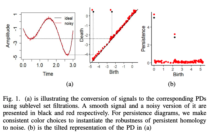

The Bayesian Model

Prior knowledge is modeled by a persistence diagram $D_X$ generated by a PPP $\mathcal{D}_X$ with intensity $\lambda_{\mathcal{D}_X}$. If $x$ is in $D_X$ but not observed in the data, we assign this event the probability $1-\alpha(x)$. Data is encoded into the observed PDs $D_Y$, and points $y_i \in D_Y$ are linked to points in $D_X$ via the MPPP. A further PPP $\mathcal{D}_{Y_U}$ with intensity $\lambda_{\mathcal{D}_{Y_U}}$ must be defined for data not associated with points in the prior.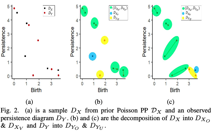

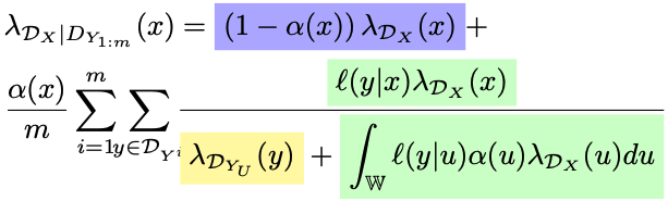
The Posterior

The first term is for features of prior that may not be observed and the second one is for features that may. Note the normalizing constant, it includes the intensity of features not associated with the prior.

Bayesian Classification

For training sets $Q_{Y^k} := D_{Y^k_{1:n}}, \ k=1, \dots, K$, we obtain the posterior density of $D|Q_{Y^k}$: $$p_{\mathcal{D}|\mathcal{D}_{Y^k}}(D|Q_{Y^k}) = \frac{e^{-\lambda}}{|D|!}\prod\limits_{d \in D} \lambda_{D|Q_{Y^k}}(d),$$ where $\lambda = \int \lambda_{D|Q_{Y^k}}(u)du$, that is the expected number of points in $D|Q_{Y^k}$.

Bayesian Classification

Analogously, we obtain posterior probability densities for other training sets and define the Bayes factor as$$BF^{i,j}(Q_{Y^i}, Q_{Y^j}) = \frac{p_{\mathcal{D}|\mathcal{D}_{Y^i}}(D|Q_{Y^i})}{p_{\mathcal{D}|\mathcal{D}_{Y^j}}(D|Q_{Y^j})},$$ for ever pair $1 \leq i, j \leq K$. If $BF^{i,j}(Q_{Y^i}, Q_{Y^j}) > c$, then one vote is assigned to class $Q_{Y^i}$, or otherwise if it is less than $c$. The class for $D$ is the one that wins by majority vote.

Conjugate Family of Priors

For a closed form of the posterior, Gaussian mixtures are chosen as a family of priors. The prior intensity density is $\lambda_{\mathcal{D}_X}(x) = \sum_{j=1}^Nc_j^{\mathcal{D}_X}\mathcal{N}^*(x; \mu_j^{\mathcal{D}_X}, \sigma_j^{\mathcal{D}_X}I)$ where $N$ is the number of mixture components and $\mathcal{N}^*$ is the restricted Gaussian on the set of birth and persistance points. $\lambda_{\mathcal{D}_{Y_U}}(y)$ is similarly defined.

Conjugate Family of Priors

The likelihood density is also Gaussian: $\ell(y|x) = \mathcal{N}^*(y; x, \sigma^{\mathcal{D}_{Y_O}}I)$, and we let $\alpha(x) = \alpha$. Thus we obtain the Gaussian mixture for the posterior intensity: $$\lambda_{\mathcal{D}_X|D_{Y_{1:n}}}(x) = (1-\alpha)\lambda_{\mathcal{D}_X}(x)$$ $$+ \frac{\alpha}{n}\sum\limits_{i=1}^n\sum\limits_{y \in \mathcal{D}_Y}\sum\limits_{j=1}^NC_j^{x|y}\mathcal{N}^*(x; \mu_j^{x|y}, \sigma_j^{x|y}I),$$ where $C_j^{x|y}$, $\mu_j^{x|y}$ and $\sigma_j^{x|y}$ are the weights mean and variance of the posterior intensity respectively.

EEG Datasets

• US Army Aberdeen Proving Ground simulated noisy EEG signals based on different activities.
• Results for alpha and beta bands are presented, where the authors describe alpha as intense activity and beta as more focused activity (maybe they meant beta and gamma respectively).

EEG Datasets

Posterior intensity estimation of a noisy alpha band and a noisy beta band. Authors employed an uninformative prior of the form $\mathcal{N}((3, 3), 20I)$. Intensities were scaled by dividing them by their corresponding maxima.

EEG Datasets

The math: everything so far. The software package: Bayes TDA. Other details: 10-fold cross validation for estimating the accuracy, each class was partitioned into 10 sets: 9 training and 1 test. Every partition was tested once. The average was taken. The results were compared to other methods: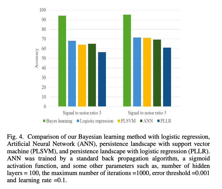

TDA is a useful and formidable tool for statisticians!

Learn more!

• A Bayesian Framework for Persistent Homology by Maroulas et al.
• Bayesian Topological Signal Processing by Oballe et al.
• Persistent Homology: a step-by-step introduction for newcomers by Fugacci et al.
• Introduction to TDA: Sources by Peter Bubenik

Questions, comments, brain waves?