Under Covers with the Mapper
Transforming High-Dimensional Data into Actionable InsightsFabiana Ferracina
July 18th, 2025
About Me and My Research
- MS in Optimization from UW, PhD in Statistics from WSU
- Past projects: burbank (potato classification framework), quantification of social cost due to travel time and carbon emissions by vehicle type, graph-based learning of aerosol dynamics (GLAD)
- Current projects: temperature effects on amorphous copper, quantifying particles from cryo-electron tomographs, image classification for ARDS diagnosis, optimization of bus routes, TDA + knot theory framework, G-RIPS coordination
Topological Data Analysis (TDA)
TDA
- Core Concept: Study the "shape" of data beyond traditional statistics
- Key Insight: Data has intrinsic geometric and topological structure
- Applications: Reveals hidden patterns, clusters, and relationships
- Advantage: Robust to noise and coordinate-free
Core Ideas
- Persistent Homology: quantifies the birth and death of topological features—such as connected components, loops, and voids—across multiple spatial or parameter scales
- Mapper: transforms high-dimensional data into a simplified graph
Core Ideas
- Persistent Homology: quantifies the birth and death of topological features—such as connected components, loops, and voids—across multiple spatial or parameter scales
- Mapper: transforms high-dimensional data into a simplified graph
The Mapper Algorithm
What it does:
- Constructs simplified topological graphs from high-dimensional data
- Preserves essential structural information
- Enables visualization of complex datasets
Key Innovation:
Transforms the challenge of understanding high-dimensional data into graph analysis - a more intuitive domain for human interpretation
Mathematical Framework
Theoretical Foundation
Given: Dataset \( X \subset \mathbb{R}^n \) and filter function \( f: X \to \mathbb{R}^d \)
Reeb Graph Connection
- Level sets: \( f^{-1}(c) = \{ m \in M \mid f(m) = c \} \)
- Connected components → nodes
- Mapper approximates Reeb graph
Nerve Complex Construction
- Cover \( U = \{ U_i \}_{i \in I} \) of \( f(X) \)
- Pullback: \( f^{-1}(U_i) \)
- Nerve: \( N(f^{-1}(U)) \) captures intersections
The Four-Step Mapper Process
- Filter Function Selection
\( f: X \to \mathbb{R}^d \) projects data to lower dimensions: PCA (most common - 47% usage), t-SNE, UMAP, MDS, domain-specific functions, etc
- Cover Construction
Create overlapping intervals \(U_i\) covering \(f(X)\): uniform vs. balanced covers. Overlap percentage (typically 20-50%). Adaptive methods emerging.
- Clustering
Cluster points in \(f^{-1}(U_i)\) for each interval: HACA (most popular), DBSCAN (density-based), custom algorithms
- Graph Construction
Connect clusters sharing data points: nodes = clusters, edges = shared points \(\Rightarrow\) topological graph \(G = (N, E)\)
Point Clouds & Preprocessing
- Load 3D data (Eagle, Knots, Synthetic)
- Downsample with voxel grids
- Normalize each cloud (centering, scaling)
Lenses: Mapping High-Dimensional Data
- PCA lens: Principal Component Analysis for linear features
- UMAP lens: Nonlinear manifold projection for shape-driven features
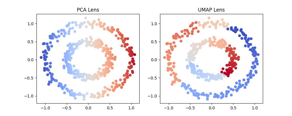
Visualization: PCA
Visualization: UMAP
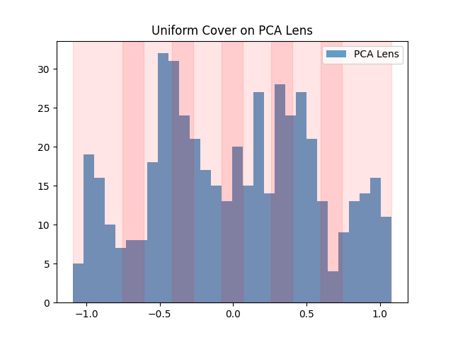
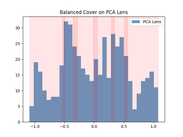
Covers: Slicing Data for Mapper
- Uniform cover: Evenly spaced, overlapping intervals on lens
- Balanced cover: Intervals contain similar data counts
- Adaptive cover: Data-driven intervals via BIC or persistent homology
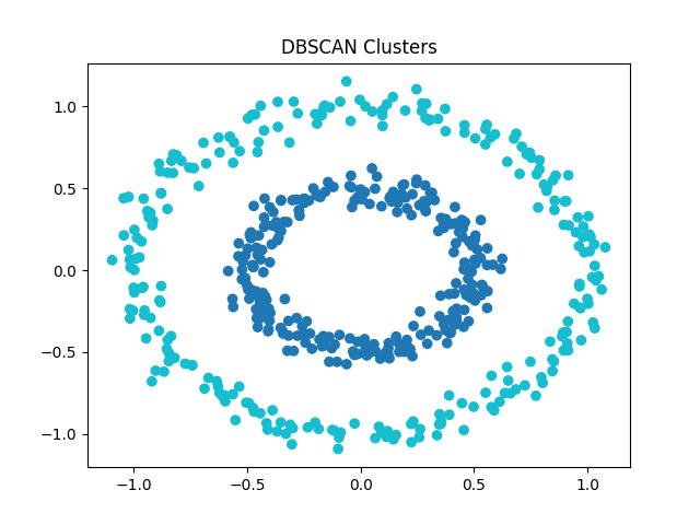
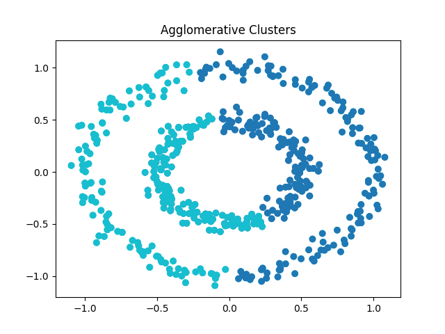
Clustering in Mapper
- Each cover slice: cluster points, form graph nodes
- Clusterers: DBSCAN (density), Agglomerative (HACA)
Mapper Pipeline
- Build lens (PCA/UMAP)
- Select cover (uniform, balanced, adaptive)
- Cluster each interval
- Build graph with adjacency by overlapping clusters
- Visualize with KeplerMapper
Mapper Pipeline
Mapper Pipeline
Algorithmic Advances and Variants
Distribution-Guided Approaches
- D-Mapper (2025): Probabilistic model-based covers using mixture models
- Adaptive Covers: Information criteria (AIC/BIC) for parameter selection
- Statistical Frameworks: Rigorous convergence guarantees
Algorithmic Advances and Variants
Ball Mapper
- Innovation: Single parameter (radius)
- Advantage: Simplified implementation
- Applications: Finance, biology, air quality
- Trade-off: Less interpretability
Algorithmic Advances and Variants
F-Mapper & V-Mapper
- F-Mapper: Fuzzy c-means for adaptive intervals
- V-Mapper: RNA velocity integration for temporal dynamics
- Benefit: Data-driven parameter selection
Algorithmic Advances and Variants
Specialized Variants
- G-Mapper: G-means clustering with Anderson-Darling test
- MEPHCA: Classification-optimized for reduced computational cost
- Two-Tier Mapper: Hierarchical + partitioning clustering
Weisfeiler-Lehman Graph Kernels in TDA
Weisfeiler-Lehman Fundamentals
- Graph Isomorphism Test: Structural similarity measurement
- Kernel Definition: \( K(G, G') = \sum_{i=0}^h \sum_{v \in V} \sum_{v' \in V'} \delta(\phi_i(v), \phi_i(v')) \)
- Subtree Features: Rapid feature extraction scheme
Weisfeiler-Lehman Graph Kernels in TDA
TDA Integration Opportunities
- Mapper Graph Comparison: Quantify topological similarity
- Persistent WL: Augment with topological information
- Graph Classification: Enhanced predictive performance
Weisfeiler-Lehman Graph Kernels in TDA
Potential Applications
- Mapper Stability Analysis: Compare graphs across parameter settings
- Ensemble Selection: Choose optimal Mapper variants
- Temporal Analysis: Track topological evolution over time
The Weisfeiler-Lehman Test
Core Concept
- Graph Isomorphism Test: Determines if two graphs are structurally identical
- Color Refinement: Iteratively assigns colors to nodes based on neighborhood structure
- Canonical Form: Creates unique representations for graph equivalence classes
Algorithm Steps
- Initialize: Assign colors to nodes based on degree
- Refine: Update colors based on neighbor colors
- Iterate: Repeat until convergence
- Compare: Test equivalence via color histograms
Mathematical Framework
Given graphs \(G_1, G_2 \) with WL equivalence, construct covers \(U_1, U_2\) such that:
- Color refinement is preserved: \(WL(G_1) \cong WL(G_2) \Rightarrow \mathrm{Mapper}(G_1, U_1) \cong \mathrm{Mapper}(G_2, U_2)\)
- Permutation invariance: \(\sigma(G)\) produces equivalent Mapper output
WL-Based Cover Construction Strategies
Density-Sensitive Integration
- Local Structure Awareness: Adapt cover density to graph connectivity
- Kernel-Based Approaches: Weight cover elements by structural similarity
- Adaptive Refinement: Dynamic adjustment based on WL convergence
WL-Based Cover Construction Strategies
Implementation Considerations
- Computational Complexity: O(n log n) per WL iteration, manageable for 2D graphs
- Memory Efficiency: Sparse representation for large graph datasets
- Scalability: Parallel processing of cover construction
WL-Mapper: Strengths and Challenges
Key Advantages
- Structural Preservation: Maintains graph isomorphism properties
- Interpretability: Clear connection between graph structure and topology
- Scalability: Polynomial-time complexity for most graphs
- Robustness: Stable under graph perturbations
WL-Mapper: Strengths and Challenges
Current Limitations
- WL Hierarchy: Cannot distinguish all non-isomorphic graphs
- Implementation Gap: Limited software support for WL-covers
- Parameter Sensitivity: Cover construction still requires tuning
- Validation: Limited empirical studies on real-world data
Applications: Knots and Bus GPS
Knotty Mapper
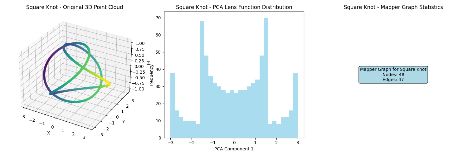
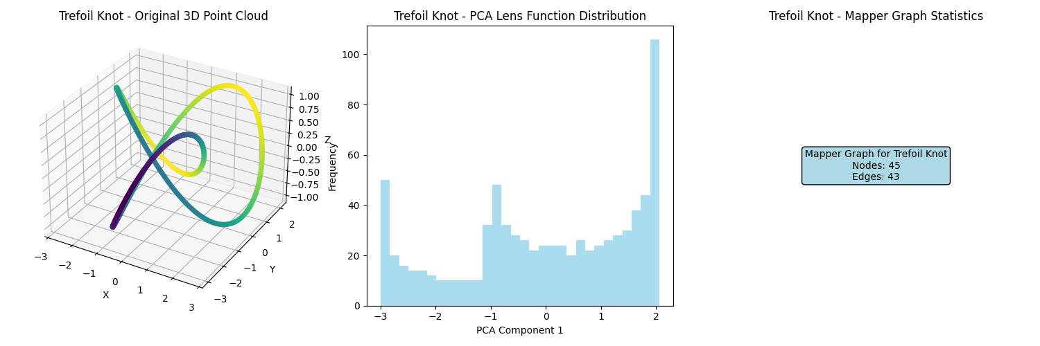
Mapper for Knot Data
Knot Mapper Classifier: PCA+DBSCAN
| Class | Precision | Recall | F1-score | Support |
|---|---|---|---|---|
| knot0009 | 1.00 | 1.00 | 1.00 | 28 |
| knot0020 | 0.92 | 1.00 | 0.96 | 24 |
| knot0021 | 1.00 | 0.80 | 0.89 | 10 |
| knot0034 | 1.00 | 0.92 | 0.96 | 24 |
| knot0035 | 0.88 | 1.00 | 0.93 | 14 |
| accuracy | 0.96 | 100 | ||
| macro avg | 0.96 | 0.94 | 0.95 | 100 |
| weighted avg | 0.96 | 0.96 | 0.96 | 100 |
WL-based Mapper for Knot Classification
| Class | Precision | Recall | F1-score | Support |
|---|---|---|---|---|
| knot0009 | 1.00 | 0.60 | 0.75 | 25 |
| knot0020 | 1.00 | 1.00 | 1.00 | 25 |
| knot0021 | 1.00 | 1.00 | 1.00 | 25 |
| knot0034 | 1.00 | 0.96 | 0.98 | 25 |
| knot0035 | 0.69 | 1.00 | 0.82 | 25 |
| accuracy | 0.91 | 125 | ||
| macro avg | 0.94 | 0.91 | 0.91 | 125 |
| weighted avg | 0.94 | 0.91 | 0.91 | 125 |
Visualization: Interactive Bus Routing
Get in the Mapper Bus
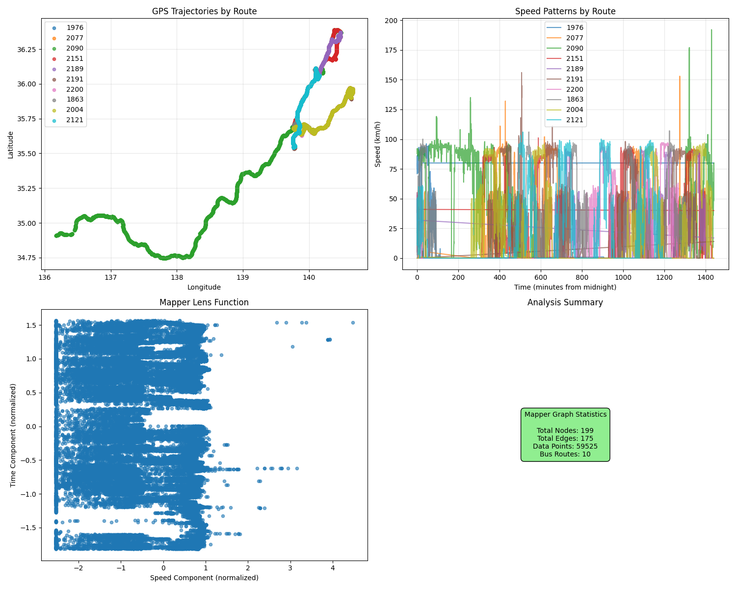
Mapper for GPS Data
Results Coming Soon
Open Research Problems and Limitations
Technical Challenges
- Parameter Sensitivity: High sensitivity to filter function and cover choices
- Automatic Selection: Need for principled parameter optimization
- Global Structure Loss: Potential loss of critical topological features
- Interpretability: Lack of standardized evaluation metrics
Open Research Problems and Limitations
Scalability Limitations
- Memory Constraints: Large dataset processing limitations
- Computational Complexity: Quadratic scaling in some variants
- Real-time Processing: Streaming data challenges
Open Research Problems and Limitations
Theoretical Gaps
- Convergence Guarantees: Limited theoretical bounds for Mapper-Reeb graph relationship
- Stability Analysis: Need for robust statistical frameworks
- Multi-scale Extensions: Hierarchical and temporal data challenges