Previously in Hidden Connections

Inspired by the idea that one can relate forest fires to neuronal spikes.

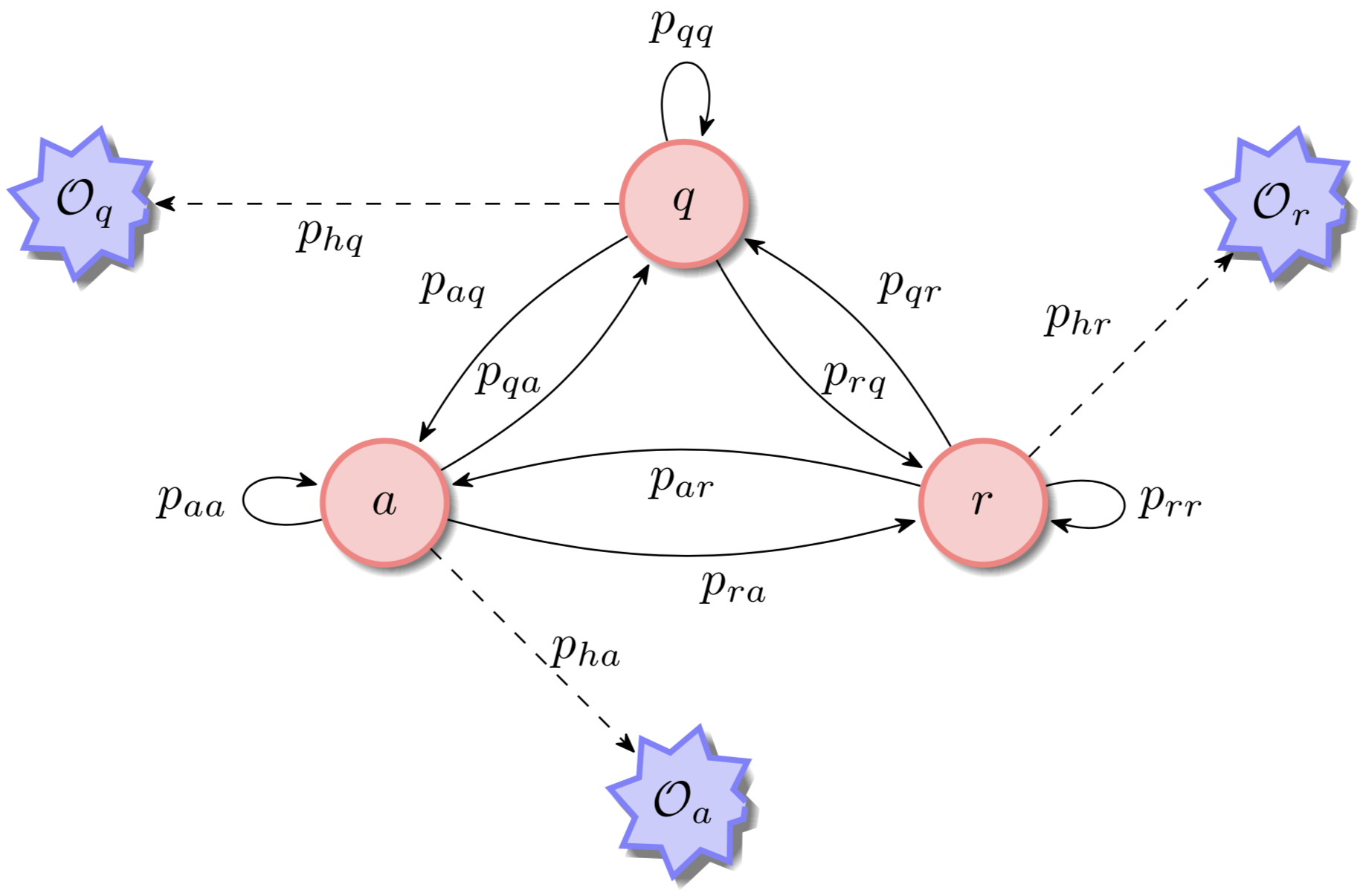
• DTMC with three states: active, refractory, quiescent.
• HMM with observed thermal readings labeled fire or no fire.
• We have a transition prob. matrix $P$, a observed$\rightarrow$state prob. matrix $B$ and an initial state vector $\pi$.
• We wish to find the model $\lambda = (P, B, \pi)$ that maximizes the likelihood of the given observation sequence.

The Data

• NASA's satellites Aqua and Terra payload MODIS, as before.
• Lower spatial resolution than before: 1 km$^2$ per pixel.
• But we get more frequent images! 1 for each day of the year.
• The place is still the Western Amazon. Two data sets: 2010 and 2019.

The Data

The higher temporal resolution makes the data is too sparse. Thus we decreased it to 5 days per time step. We also decreased the spatial to 10 km$^2/$pixel.

The Network Model

A Network of HMMs

Each node in the network is an HMM like decribed before.

How Transitions Work

As an example consider a node $C$ with transition probabilities matrix $P_0$ at time $t=0$.

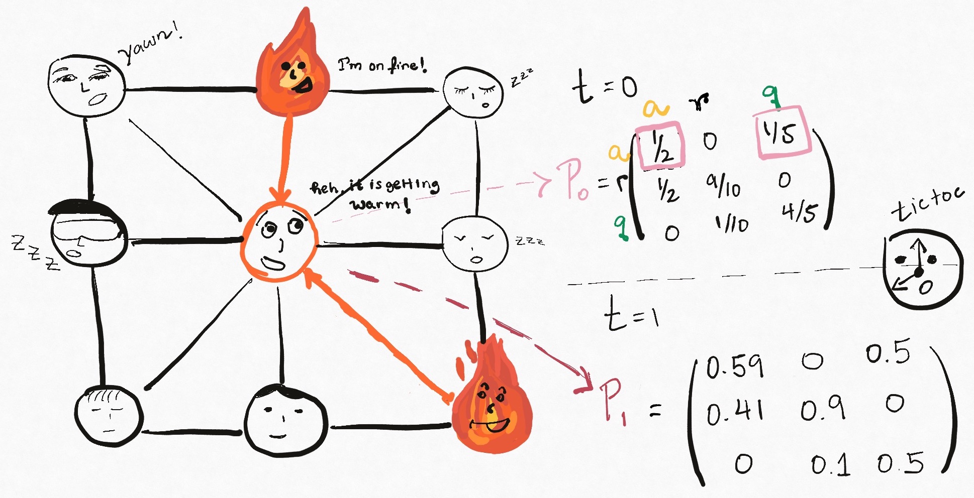(multipliers for $[a \rightarrow a]$ and $[q \rightarrow a]$ are 1.2 and 2.0, respectively.)

If $C$ is adjacent to two active nodes at $t=0$, then at $t=1$ its transition probalities matrix becomes $P_1$.

HMM Implementation: Same as Before

Initial Pre-chosen Values:

Solve for $\lambda$ with Baum-Welch algorithm.

$\alpha$'s, $\beta$'s and MSE's

However, within a spatial 2D network, we further update the transition probabilities matrix $P$ for each node in the network (e.g a patch of land), at each time step, conditional on the states of the neighboring nodes.

These updates occur as newly introduced weights $\alpha$ and $\beta$, which are applied to the states $a \rightarrow a$ and $q \rightarrow a$ of the transition matrix $P$ for each node at each time step.

Wait!...the MSE's?

We run a Monte Carlo simulation to find the $(\alpha, \beta)$ pair that minimizes the mean squared error (MSE) of the fire density in our training dataset. For example, here are 25 such pairs and their corresponding MSE's:

Fitted Transition Probabilities

Results

$\alpha = 1, \beta = 10$: adjacent quiecents get more affected.

Results

$\alpha = 2, \beta = 10$: active nodes and adjacent quiecents get more affected.

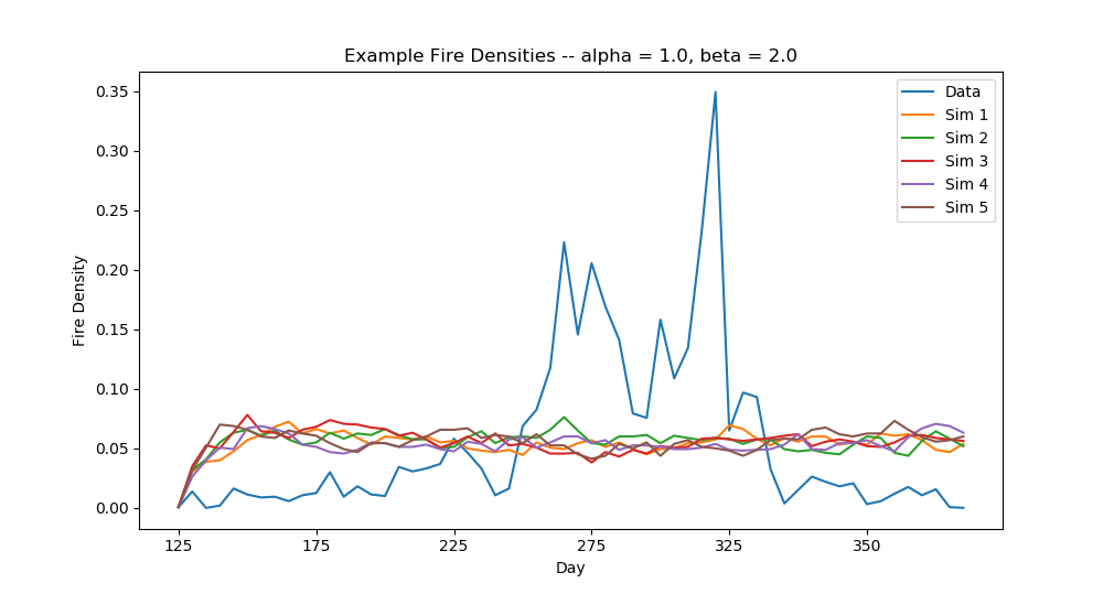
Results

$\alpha = 2, \beta = 2$: active nodes and adjacent quiecents get more affected.

Results

$\alpha = 1, \beta = 2$: best multipliers.

(left: low resolution version of training data, right: the results)

Results

However, we still have a long way to go...

Importance

If we can predict fire spread and magnitude from earlier remote sensed data:

• We can fight it with the appropriate response later.
• We can investigate problem areas and come up with mitigation responses.
• If we can modify the vegetation in order to prevent large escalations.
• We can evacuate animal and human inhabitants before it is too late.

Thank you!