Topological Data Analysis of Urban Bus Networks
Persistent Homology on Multi-View Heatmaps for Operational InsightsFabiana Ferracina (Tohoku University)
December 14th, 2025
Operational Question
Several routes have been suffering delays due to temporal bunching. We would like to implement bunching mitigation efficiently by adding holding times at control points.
Motivation and OR Context
- Urban bus systems are typically analyzed via averages: mean speed, headway variance, load factors.
- Different routes can share similar averages yet behave very differently operationally.
- Operations research models need structure: where do we see skip-stop, bunching, or fragile patterns?
- Topological Data Analysis (TDA) summarizes the shape of traffic fields, not just their level.
Data and Study Setting
Data: Large-Scale Bus GPS Operations
- Operator: Kanto Railway (regional bus company in Japan).
- Period: 247 days (Jan–Sep 2020), including pre-pandemic and pandemic adjustments.
- Scale: 290,441 vehicle-days across 460 distinct routes.
- Per record: latitude, longitude, timestamp, instantaneous speed, heading, route ID, passenger count.
Example Route-Day
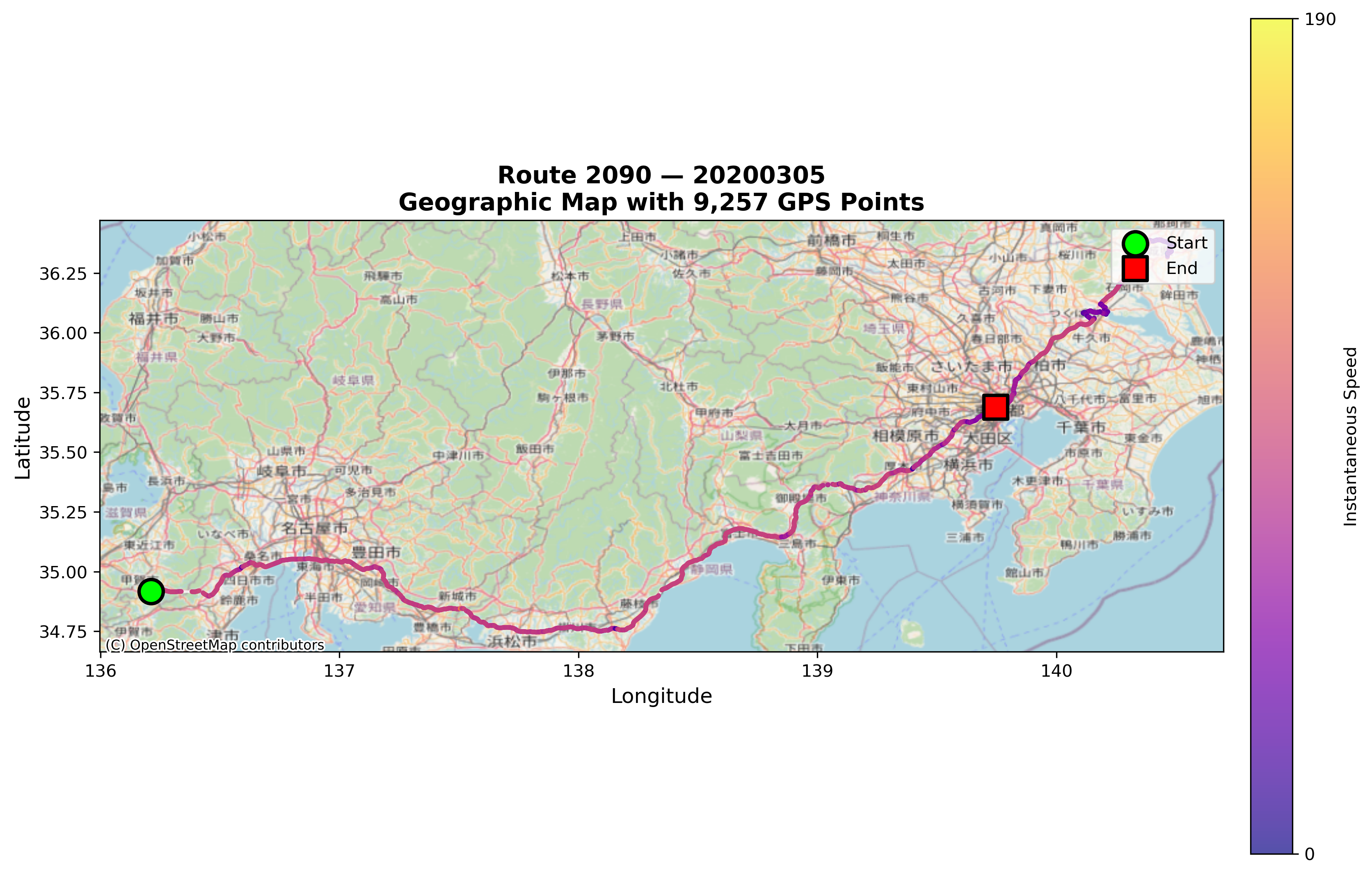 GPS trajectory color-coded by speed. Pink-to-yellow segments: high-speed highway operation; pink-to-blue: deceleration near stops or congestion.
This spatial alternation is what will later generate complex topological patterns.
GPS trajectory color-coded by speed. Pink-to-yellow segments: high-speed highway operation; pink-to-blue: deceleration near stops or congestion.
This spatial alternation is what will later generate complex topological patterns.
GPS \(\rightarrow\) Multi-View Heatmaps
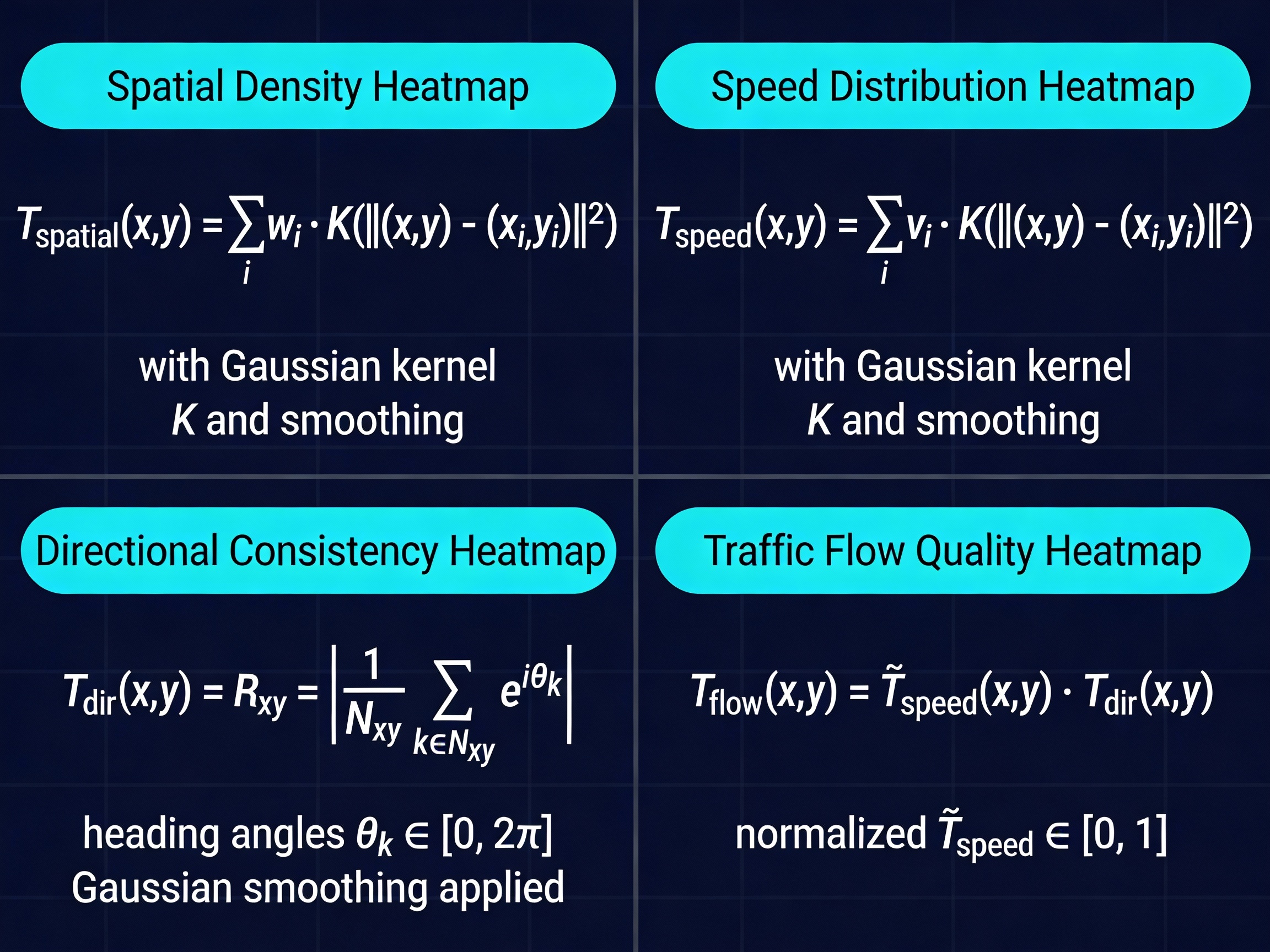 Spatial density: where vehicles spend time. Speed distribution: where they slow down vs. cruise.
Directional consistency: how coherent the flow direction is. Traffic flow quality: speed ×
directional coherence.
Spatial density: where vehicles spend time. Speed distribution: where they slow down vs. cruise.
Directional consistency: how coherent the flow direction is. Traffic flow quality: speed ×
directional coherence.
Computational Pipeline
 Pipeline: GPS trajectories → heatmap on grid → cubical complex filtration → persistence diagram
→ summary statistics. This runs independently on all four heatmap views.
Pipeline: GPS trajectories → heatmap on grid → cubical complex filtration → persistence diagram
→ summary statistics. This runs independently on all four heatmap views.
Intuition: What Does Persistent Homology Measure?
- Think of a heatmap as a landscape: low values are valleys, high values are hills.
- We gradually “flood” this landscape and track how connected regions and loops appear/disappear.
- H0: number of connected components → fragmented coverage or multiple congestion zones.
- H1: number of loops/cycles → rings of high/low flow, indicative of skip-stop or complex patterns.
Persistent Homology
Persistent Homology and Diagrams
For a single variate function, such as the signal below, we can track and encode the evolution of connected components (0-d homology) of its sublevel-sets:
source
Persistent Homology and Diagrams
Note that we track the components for each $f^{-1}((-\infty, \alpha])$ where $\alpha \in (-\infty, \infty)$. Below we see that components are born at local minima and die at local maxima: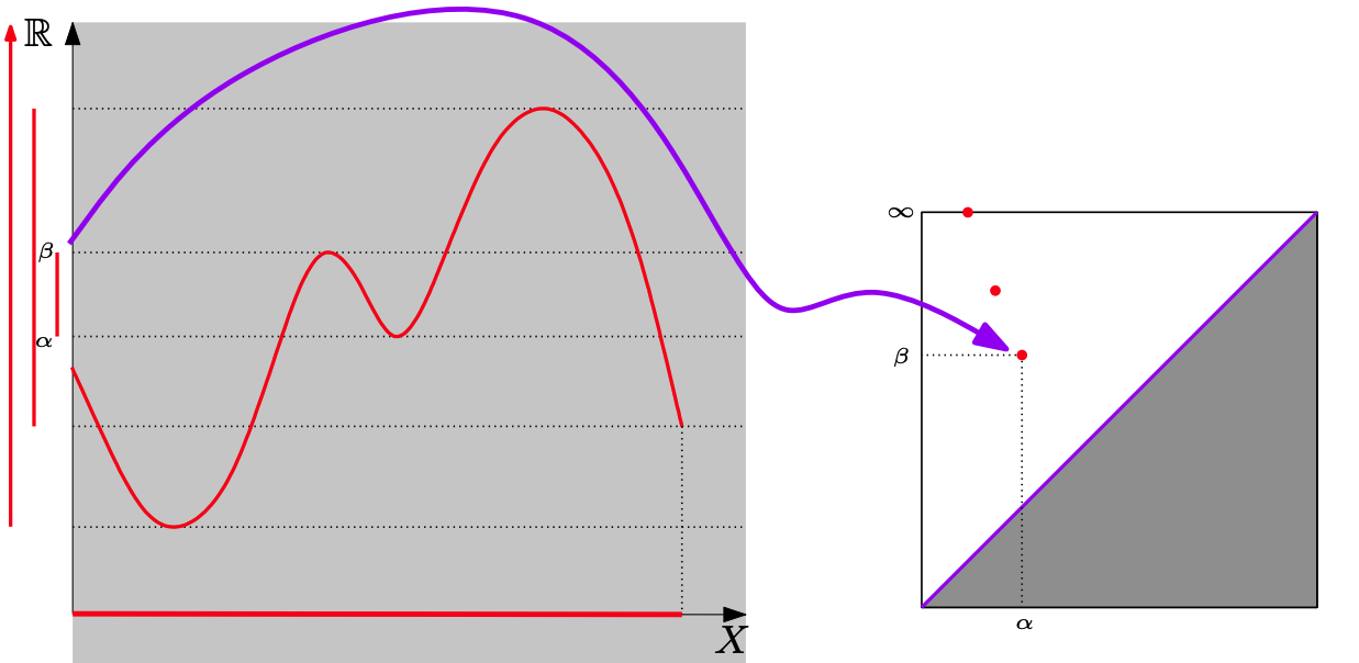
source
Route-Level Feature Summary
- Conventional: mean speed, speed standard deviation, congestion fraction.
- Topological: counts of H0, H1 features in spatial and flow views.
- Strong right-skew: most routes have simple flow topology; a subset exhibits very high complexity.
- This suggests natural route categories rather than a single homogeneous class.
- Low correlation between speed and flow H1 indicates that topology captures information beyond basic kinematics.
Unsupervised Route Clustering
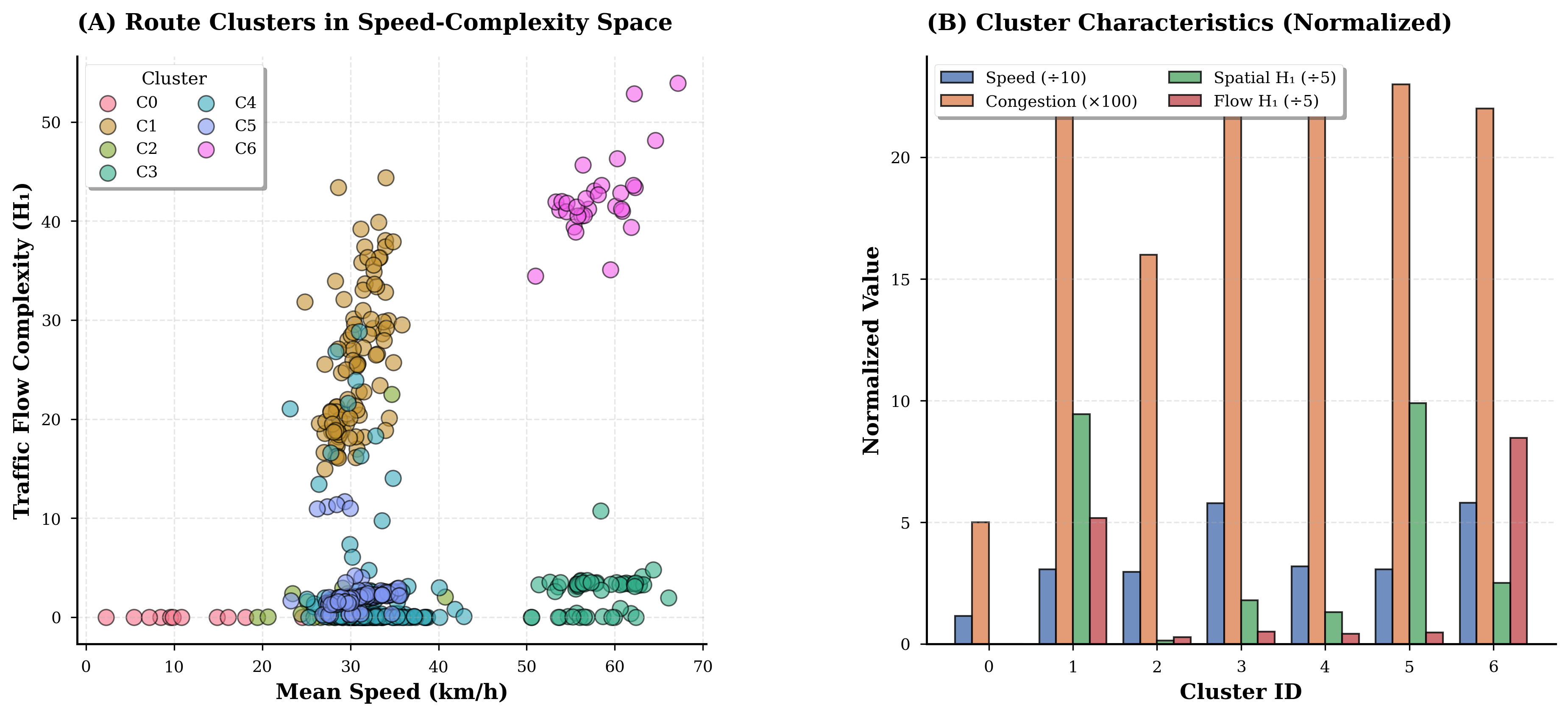 k-means on standardized features (speed, congestion, spatial H1, flow H1) reveals seven
operationally distinct clusters; silhouette analysis supports k = 7.
k-means on standardized features (speed, congestion, spatial H1, flow H1) reveals seven
operationally distinct clusters; silhouette analysis supports k = 7.
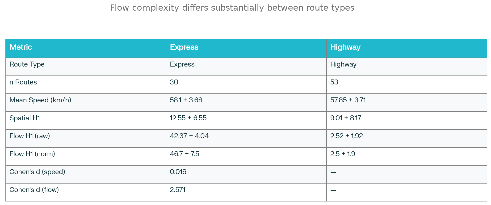
Two High-Speed Worlds: Express vs Highway
- Cluster 3: “Highway” — high speed, low flow complexity, simple topology.
- Cluster 6: “Express” — similarly high speed, but extremely high flow complexity.
- Key result: mean speeds ~58 km/h in both clusters (Cohen’s d ≈ 0.016).
- Normalized flow H1 differs by a factor of 18.4 per 1000 GPS points.
- This operational gap is invisible to conventional averages but critical for planning.
Express vs Highway
 Spatial geometry explains gap? No. (1.4-fold vs 18.4-fold)
Temporal Bunching vs Flow Topology
- Hawkes process on arrival events at a reference location captures temporal self-excitation (bunching).
- Highway routes: stronger temporal clustering (branch ratio, self-excitation parameter higher).
- Express routes: weaker temporal clustering, but far more complex flow topology.
- Conclusion: temporal bunching and topological complexity are orthogonal dimensions.
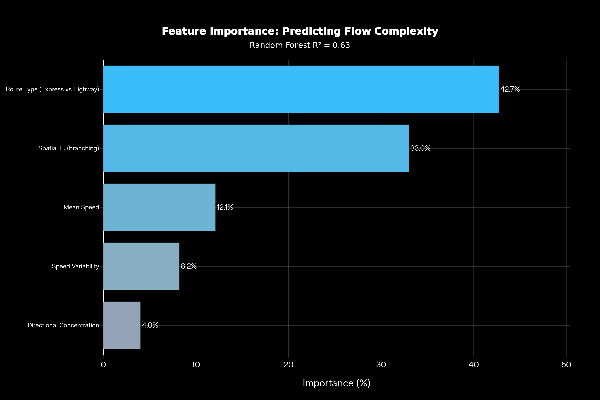
What Drives Topological Complexity?
How Does This Relate to OR Models?
- Classical OR: p-median, MIP network design, and timetable optimization assume objectives are known.
- TDA plays a complementary role: it discovers latent structure in operations from raw data.
- Example: the 18.4× Express–Highway complexity gap suggests differentiated objective functions.
- For Express routes: constrain flow complexity; for Highway routes: prioritize bunching control.
Utility, Fairness, and Practical Use
- Utility: identify routes with complex flow topology that may be fragile or confusing to riders.
- Fairness: combine topological indicators with demand to find “transit deserts” and overloaded corridors.
- Usefulness: route-type-specific policies (Express vs Highway) instead of one-size-fits-all service rules.
- All built on data operators already collect, with scalable computation.
Limitations and Next Steps
- Single operator and region; need cross-city and cross-mode validation.
- Current analysis focuses on geometry and kinematics, not passenger demand.
- Persistent homology is descriptive; integrating it with optimization remains an open OR problem.
- Future: demand-weighted topology, Mapper-based trajectory graphs, topology-constrained network design.
TDA offers OR practitioners a discovery layer to inform fairness-aware, route-type-specific policies.
Thank you!
Extra Slides
Why a Composite Flow Metric?
- Raw speed persistence generates many short-lived loops (mean ≈ 215.5 H1 features).
- These loops largely reflect transient speed fluctuations rather than stable operational patterns.
- Multiplying normalized speed by directional consistency suppresses noisy regions.
- Only locations with both high speed and coherent direction produce strong traffic flow quality signals.
- Downstream clustering therefore uses flow H1 rather than speed H1 as the primary topological feature.
Length-Normalized and Decomposition Results
- Normalizing by GPS point density controls for route length and sampling frequency.
- Express routes maintain higher complexity per unit length; ratio increases from 16.8× to 18.4×.
- Decomposition of Qflow into speed and directional components clarifies mechanism.
- Within routes, flow H1 correlates strongly with directional consistency H1 (ρ ≈ 0.89).
- Correlation with speed-derived topology is weak (ρ ≈ 0.17), indicating directional heterogeneity in routing geometry drives complexity.
Topology Mismatch: Two Distinct Regimes
Flow-Dominant
High Flow H₁ complexity
Low Spatial H₁ (simple geometry)
Example: Express skip-stop routes
d = 10.17 (massive effect)
Spatial-Dominant
High Spatial H₁ (complex branching)
Low Flow H₁ complexity
Example: Multi-branch uniform routes
d = 4.35 (large effect)
Take-Home Messages
- Multi-view heatmaps and cubical persistent homology reveal operational structures hidden from averages.
- Two high-speed route types differ 18.4× in flow complexity despite identical mean speeds.
- Topological features are robust, interpretable, and orthogonal to temporal bunching.
- TDA offers OR practitioners a discovery layer to inform fairness-aware, route-type-specific policies.
About this research:
- G-RIPS Sendai internship in 2022: QBD process using Kanto area person-trip data. (Nakamura et al.)
- Statistics Ph.D. from WSU, now Assistant Professor at Tohoku University.
- New team: Ayane Nakamura (Keio University), Hiroyasu Ando (Tohoku University), Bala Krishnamoorthy (WSU), myself.
- Large GPS dataset, many interesting questions.